Day 9 Communicating results
February 9th, 2026
9.1 Scientific writing
- Introduction
- More general –> more specific
- Last paragraph states the knowledge gap, and clearly mentions objectives.
- Using wording like “the objectives were …”

- M&M
- Reproducibility
- Reproducibility of the experiment
- Reproducibility of the statistical model
- Reproducible environments
- Results
- Highlight important results
- Discussion
- Put results in context
- Conclusion
- Connect the topic sentences in the discussion
- Writing Center (KSU)
- Writing scientific papers
9.1.1 Paragraphs
- One idea per paragraph
- One (bigger) idea per paper
- Structure of a paragraph [link to resource]
- Topic sentence - presents the idea/claim of the paragraph
- Evidence
- Analysis
- Conclusion

9.2 Communicating statistical analyses
- Discipline-specific criteria
- Statistical notation versus rhetoric
Some examples from this class.
9.3 Communicating results and uncertainty
Communicating point estimates is relatively easy. So far, we can consider the point estimate the value with maximum likelihood to have generated the data. If we had to bet on a particular number, that would probably be the point estimate. Now, if we had to bet on a range of values, the width of that range would depend on the information in the data.
Confidence intervals
Confidence intervals are one of the most frequently mis-interpreted quantities.
- A safe approach: “The mean is between
CIlowandCIhigh[units], with 95% confidence.” - Statistical tests, P values, confidence intervals, and power: a guide to misinterpretation [link to paper]
9.3.1 Example
The data below come from a split-plot designed experiment in complete blocks, with fungicide in the whole plot and genotype in the split plot. The model is
\[y_{ijk} | b_k, u_{j(k)} \sim N(\mu_{ijk}, \sigma^2_\varepsilon), \\ \mu_{ijk} = \mu + G_i + F_j + GF_{ij} + b_k + u_{j(k)}, \\ b_k \sim N(0, \sigma^2_b) , \ u_{j(k)} \sim N(0, \sigma^2_u),\]
where \(y_{ijk}\) is the data that we assume is normally distributed, \(\mu_{ijk}\) is the mean and \(\sigma^2_\varepsilon\) is the variance. The linear predictor of \(\mu_{ijk}\) is the sum of an overall mean \(\mu\), the effect of the \(i\)th genotype \(G_i\), the effect of the \(j\)th fungicide \(F_j\), the interaction between the \(i\)th genotype and \(j\)th fungicide \(GF_{ij}\), the random effect of the \(k\)th block \(b_k\), and the random whole-plot effect of the \(j\)th fungicide in the \(k\)th block \(u_{j(k)}\). Both random effects are assumed independent to each other and to the residual.
dat_multilevel <- agridat::durban.splitplot

m_multilevel <- lmer(yield ~ gen*fung + (1|block/fung), data = dat_multilevel)

fung_mgmeans <- emmeans(m_multilevel, ~fung)
## NOTE: Results may be misleading due to involvement in interactionsas.data.frame(fung_mgmeans) |>
ggplot(aes(emmean, fung))+
geom_errorbarh(aes(xmin = lower.CL, xmax = upper.CL), width = 0)+
geom_point(size = 4)+
theme_bw()+
labs(y = "Fungicide", x = expression(Yield~(Mg~ha^{-1})))+
theme(aspect.ratio = .2)## Warning: `geom_errorbarh()` was deprecated in ggplot2 4.0.0.
## ℹ Please use the `orientation` argument of `geom_errorbar()` instead.
## This warning is displayed once per session.
## Call `lifecycle::last_lifecycle_warnings()` to see where this warning was generated.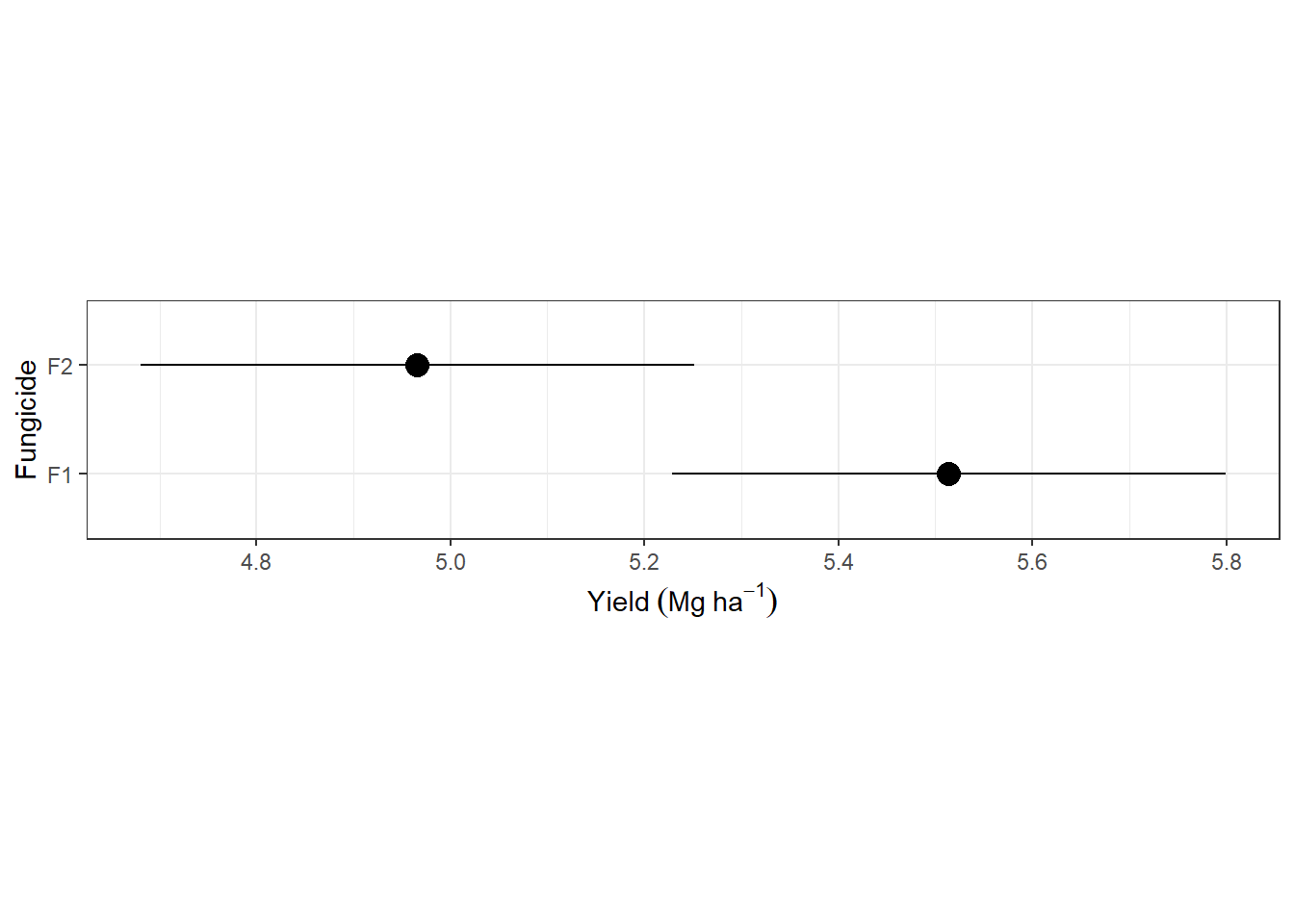
9.3.2 Hypothesis tests and p-values
Hypothesis test evaluate the probability of observing the current data under a null hypothesis. When that probability is very low, we consider that is it very unlikely that the data were generated by that hypothesis, and we move on to an alternative hypothesis.
What we need:
- A null hypothesis \(H_0\) representing the current paradigm or beliefs
- An alternative hypothesis \(H_a\)
What we get:
- An answer rejecting (or not) the null hypothesis.
Things to consider:
- The question reflected in some \(H_0\) is not always the real research question.
- The Difference Between “Significant” and “Not Significant” is not Itself Statistically Significant [link to paper]
- ASA’s statement on p-values [link to paper]
Different types of hypothesis tests
- t-tests
- ANOVA – F test ~ multivariate t-test
- Post-hoc mean comparisons
## $emmeans
##  fung emmean    SE   df lower.CL upper.CL
##  F1     5.51 0.105 4.18     5.23     5.80
##  F2     4.97 0.105 4.18     4.68     5.25
##
## Results are averaged over the levels of: gen
## Degrees-of-freedom method: kenward-roger
## Confidence level used: 0.95
##
## $contrasts
##  contrast estimate     SE df t.ratio p.value
##  c(1, -1)    0.548 0.0863  3   6.346  0.0079
##
## Results are averaged over the levels of: gen
## Degrees-of-freedom method: kenward-roger## Analysis of Deviance Table (Type II Wald F tests with Kenward-Roger df)
##
## Response: yield
## F Df Df.res Pr(>F)
## gen 7.2008 69 414 < 2.2e-16 ***
## fung 40.2718 1 3 0.007915 **
## gen:fung 0.9331 69 414 0.629010
## ---
## Signif. codes: 0 '***' 0.001 '**' 0.01 '*' 0.05 '.' 0.1 ' ' 1# multiple comparison
library(multcomp)
means_gen <- emmeans(m_multilevel, ~gen)
(mean_comparisons_gen <-
cld(means_gen,
level = 0.05,
adjust = "sidak",
Letters = letters))## gen emmean SE df lower.CL upper.CL .group
## G04 4.14 0.137 12.8 3.84 4.45 a
## G14 4.63 0.137 12.8 4.32 4.94 ab
## G20 4.80 0.137 12.8 4.49 5.11 bc
## G10 4.81 0.137 12.8 4.50 5.12 bcd
## G28 4.84 0.137 12.8 4.53 5.15 bcde
## G24 4.86 0.137 12.8 4.55 5.16 bcdef
## G01 4.91 0.137 12.8 4.60 5.22 bcdefg
## G05 4.94 0.137 12.8 4.63 5.25 bcdefgh
## G49 4.95 0.137 12.8 4.64 5.26 bcdefgh
## G34 5.01 0.137 12.8 4.70 5.32 bcdefghi
## G25 5.02 0.137 12.8 4.71 5.33 bcdefghi
## G30 5.04 0.137 12.8 4.73 5.35 bcdefghi
## G21 5.05 0.137 12.8 4.74 5.36 bcdefghi
## G02 5.06 0.137 12.8 4.75 5.37 bcdefghi
## G15 5.07 0.137 12.8 4.76 5.38 bcdefghi
## G41 5.09 0.137 12.8 4.78 5.40 bcdefghi
## G08 5.09 0.137 12.8 4.78 5.40 bcdefghi
## G07 5.10 0.137 12.8 4.79 5.41 bcdefghi
## G45 5.11 0.137 12.8 4.80 5.42 bcdefghi
## G06 5.13 0.137 12.8 4.82 5.44 bcdefghi
## G55 5.14 0.137 12.8 4.83 5.45 bcdefghij
## G32 5.16 0.137 12.8 4.85 5.47 bcdefghij
## G11 5.16 0.137 12.8 4.86 5.47 bcdefghij
## G39 5.18 0.137 12.8 4.87 5.49 bcdefghij
## G61 5.20 0.137 12.8 4.89 5.51 bcdefghij
## G53 5.21 0.137 12.8 4.90 5.52 bcdefghij
## G37 5.21 0.137 12.8 4.90 5.52 bcdefghij
## G26 5.21 0.137 12.8 4.90 5.52 bcdefghij
## G43 5.21 0.137 12.8 4.91 5.52 bcdefghij
## G35 5.22 0.137 12.8 4.91 5.53 bcdefghij
## G66 5.22 0.137 12.8 4.91 5.53 bcdefghij
## G16 5.23 0.137 12.8 4.92 5.54 bcdefghij
## G68 5.25 0.137 12.8 4.94 5.56 cdefghij
## G46 5.25 0.137 12.8 4.94 5.56 cdefghij
## G29 5.26 0.137 12.8 4.95 5.57 cdefghij
## G47 5.27 0.137 12.8 4.96 5.58 cdefghij
## G44 5.29 0.137 12.8 4.98 5.60 cdefghij
## G23 5.29 0.137 12.8 4.98 5.60 cdefghij
## G56 5.29 0.137 12.8 4.99 5.60 cdefghij
## G58 5.31 0.137 12.8 5.00 5.62 cdefghij
## G57 5.32 0.137 12.8 5.01 5.62 cdefghij
## G63 5.32 0.137 12.8 5.01 5.63 cdefghij
## G62 5.32 0.137 12.8 5.01 5.63 cdefghij
## G54 5.33 0.137 12.8 5.02 5.64 cdefghij
## G51 5.36 0.137 12.8 5.05 5.67 cdefghij
## G67 5.37 0.137 12.8 5.06 5.68 cdefghij
## G42 5.37 0.137 12.8 5.06 5.68 cdefghij
## G59 5.37 0.137 12.8 5.06 5.68 cdefghij
## G22 5.37 0.137 12.8 5.06 5.68 cdefghij
## G65 5.38 0.137 12.8 5.07 5.69 cdefghij
## G69 5.38 0.137 12.8 5.07 5.69 cdefghij
## G38 5.38 0.137 12.8 5.07 5.69 cdefghij
## G12 5.39 0.137 12.8 5.08 5.70 cdefghij
## G31 5.41 0.137 12.8 5.10 5.72 defghij
## G50 5.42 0.137 12.8 5.11 5.73 efghij
## G17 5.42 0.137 12.8 5.12 5.73 efghij
## G52 5.43 0.137 12.8 5.12 5.74 efghij
## G64 5.44 0.137 12.8 5.13 5.75 efghij
## G13 5.45 0.137 12.8 5.14 5.76 fghij
## G70 5.45 0.137 12.8 5.14 5.76 fghij
## G09 5.46 0.137 12.8 5.15 5.77 fghij
## G60 5.48 0.137 12.8 5.17 5.79 ghijk
## G27 5.49 0.137 12.8 5.18 5.80 ghijk
## G18 5.50 0.137 12.8 5.19 5.81 ghijk
## G36 5.50 0.137 12.8 5.20 5.81 ghijk
## G48 5.51 0.137 12.8 5.20 5.82 ghijk
## G40 5.53 0.137 12.8 5.22 5.84 hijk
## G33 5.61 0.137 12.8 5.30 5.92 ijk
## G19 5.73 0.137 12.8 5.42 6.04 jk
## G03 6.08 0.137 12.8 5.77 6.38 k
##
## Results are averaged over the levels of: fung
## Degrees-of-freedom method: kenward-roger
## Confidence level used: 0.05
## Conf-level adjustment: sidak method for 70 estimates
## P value adjustment: sidak method for 2415 tests
## significance level used: alpha = 0.05
## NOTE: If two or more means share the same grouping symbol,
## then we cannot show them to be different.
## But we also did not show them to be the same.9.3.3 Other results in mixed-effects models
Variance components
Recall that
\[y_{ijk} | b_k, u_{j(k)} \sim N(\mu_{ijk}, \sigma^2_\varepsilon), \\ \mu_{ijk} = \mu + G_i + F_j + GF_{ij} + b_k + u_{j(k)}, \\ b_k \sim N(0, \sigma^2_b) , \ u_{j(k)} \sim N(0, \sigma^2_u) \]
represents the conditional distribution of \(y\).
At that level, the uncertainty is only coming from observing new data, \(\sigma^2_\varepsilon\). We could, however, obtain \(y\)s for all blocks and whole plots in general, where the uncertainty will represent (i) observing new data, (ii) observing new blocks, and (iii) observing new whole plots.
##  Groups     Name        Std.Dev.
##  fung:block (Intercept) 0.11737
##  block      (Intercept) 0.16972
## Residual 0.28119- Discuss marginal inference versus conditional inference.
9.4 Reading
Writing
- Draft no. 4 (John McPhee) [link to book]
- Learning how to learn (Oakley et al.) [link to book]
Data visualization
- How to get better at embracing unknowns (J Hullman) [link to article]
- “The least effective way to present uncertainty is to not show it at all.”
- Visualizing Uncertainty About the Future (Spiegelhalter et al.) [link to article]
Other
- Cross-validation strategies for data with temporal, spatial, hierarchical, or phylogenetic structure [link to article]