Day 10 Wrap-up
February 12, 2026
10.1 Announcements
- Schedule your weekly/by-weekly meeting!
- Please fill out this form by Monday midnight.
- What’s coming next:
- Meet by appointment
- Potentially schedule group meetings for common topics
10.2 From normal, iid data, to generalized mixed models
We started from the most common statistical model
\[\mathbf{y} \sim N(\boldsymbol\mu, \boldsymbol\Sigma),\]
where:
- \(\mathbf{y} \equiv [y_1, y_2, \dots, y_n]'\) contains the response data,
- \(\boldsymbol{\mu} \equiv [\mu_1, \mu_2, \dots, \mu_n]'\) contains the expected values of said data,
- \(\boldsymbol\Sigma\) is the variance-covariance matrix.
The most typical model typically has:
- \(\boldsymbol\mu = \mathbf{X}\boldsymbol{\beta}\) and
- \(\boldsymbol\Sigma = \sigma^2\mathbf{I}\).
We can write the default model in most software written above as:
\[\mathbf{y} \sim N(\boldsymbol{\mu}, \Sigma),\\ \begin{bmatrix}y_1 \\ y_2 \\ y_3 \\ y_4 \\ \vdots \\ y_n \end{bmatrix} \sim N \left( \begin{bmatrix}\mu_1 \\ \mu_2 \\ \mu_3 \\ \mu_4 \\ \vdots \\ \mu_n \end{bmatrix}, \sigma^2 \begin{bmatrix} 1 & 0 & 0 & 0 & \dots & 0 \\ 0 & 1 & 0 & 0 & \dots & 0 \\ 0 & 0 & 1 & 0 & \dots & 0 \\ 0 & 0 & 0 & 1 & \dots & 0 \\ \vdots & \vdots & \vdots & \vdots & \ddots & \vdots\\ 0 & 0 & 0 & 0 & \dots & 1 \end{bmatrix} \right),\]
which is the same as
\[\begin{bmatrix}y_1 \\ y_2 \\ y_3 \\ y_4 \\ \vdots \\ y_n \end{bmatrix} \sim N \left( \begin{bmatrix}\mu_1 \\ \mu_2 \\ \mu_3 \\ \mu_4 \\ \vdots \\ \mu_n \end{bmatrix}, \begin{bmatrix} \sigma^2 & 0 & 0 & 0 & \dots & 0 \\ 0 & \sigma^2 & 0 & 0 & \dots & 0 \\ 0 & 0 & \sigma^2 & 0 & \dots & 0 \\ 0 & 0 & 0 & \sigma^2 & \dots & 0 \\ \vdots & \vdots & \vdots & \vdots & \ddots & \vdots\\ 0 & 0 & 0 & 0 & \dots & \sigma^2 \end{bmatrix} \right).\]
In summary, the assumptions of the most common statistical model are:
- Linearity (or whatever the deterministic equation is)
- Normality
- Independence
- Constant variance
In what follows, we will discuss the different approaches we took for relaxing those assumptions.
10.2.1 Independence Mixed models!
- Include random effects!
- How can we distinguish random vs. fixed effects?
| Fixed effects | Random effects | |
|---|---|---|
| Where | Expected value (of the marginal dist) | Variance-covariance matrix (of the marginal dist) |
| Inference | Constant for all groups in the population of study | Differ from group to group |
| Usually used to model | Carefully selected treatments or genotypes | The study design (aka structure in the data, or what is similar to what) |
| Assumptions | \[\hat{\boldsymbol{\beta}} \sim N \left( \boldsymbol{\beta}, (\mathbf{X}^T \mathbf{V}^{-1} \mathbf{X})^{-1} \right) \] | \[u_j \sim N(0, \sigma^2_u)\] |
| Method of estimation | Maximum likelihood, least squares | Restricted maximum likelihood (shrinkage) |
What we get from these assumptions
- Information is shared across groups (see analysis of IBDs in day 3)
- Precision + accuracy
- Shrinkage – see distribution
Consider the conditional distribution
\[\mathbf{y} | \boldsymbol{u} \sim N(\mathbf{X}\boldsymbol{\beta} + \mathbf{Z}\boldsymbol{u}, \mathbf{R}),\]
where \(\mathbf{y}\) is the observed response, \(\mathbf{X}\) is the matrix with the explanatory variables, \(\mathbf{Z}\) is the design matrix, \(\boldsymbol{\beta}\) is the vector containing the fixed-effects parameters, \(\mathbf{u} \sim N(\boldsymbol{0}, \mathbf{G})\) is the vector containing the random effects parameters, \(\boldsymbol{\varepsilon}\) is the vector containing the residuals, \(\mathbf{G}\) is the variance-covariance matrix of the random effects, and \(\mathbf{R}\) is the variance-covariance matrix of the residuals.
Consider the marginal distribution
\[\mathbf{y} = \mathbf{X} \boldsymbol{\beta} + \mathbf{Z}\mathbf{u} + \boldsymbol{\varepsilon}, \\ \begin{bmatrix}\mathbf{u} \\ \boldsymbol{\varepsilon} \end{bmatrix} \sim \left( \begin{bmatrix}\boldsymbol{0} \\ \boldsymbol{0} \end{bmatrix}, \begin{bmatrix}\mathbf{G} & \boldsymbol{0} \\ \boldsymbol{0} & \mathbf{R} \end{bmatrix} \right),\]
where \(\mathbf{y}\) is the observed response, \(\mathbf{X}\) is the matrix with the explanatory variables, \(\mathbf{Z}\) is the design matrix, \(\boldsymbol{\beta}\) is the vector containing the fixed-effects parameters, \(\mathbf{u}\) is the vector containing the random effects parameters, \(\boldsymbol{\varepsilon}\) is the vector containing the residuals, \(\mathbf{G}\) is the variance-covariance matrix of the random effects, and \(\mathbf{R}\) is the variance-covariance matrix of the residuals. Typically, \(\mathbf{G} = \sigma^2_u \mathbf{I}\) and \(\mathbf{R} = \sigma^2 \mathbf{I}\).
- Basically, all the random effects information is now contained in a more fancy variance-covariance matrix.
- Uncertainty includes observing new levels of the random effects (new blocks, new locations, etc, etc.)
Multilevel models are everywhere
I want to convince the reader of something that appears unreasonable: multilevel regression deserves to be the default form of regression. Papers that do not use multilevel models should have to justify not using a multilevel approach. Certainly some data and contexts do not need the multilevel treatment. But most contemporary studies in the social and natural sciences, whether experimental or not, would benefit from it. Perhaps the most important reason is that even well-controlled treatments interact with unmeasured aspects of the individuals, groups, or populations studied. This leads to variation in treatment effects, in which individuals or groups vary in how they respond to the same circumstance. Multilevel models attempt to quantify the extent of this variation, as well as identify which units in the data responded in which ways.
Richard McElreath – Statistical Rethinking
10.2.3 Normality Generalized linear models
Part of creating a statistical model is picking the distribution! A few things to keep in mind:
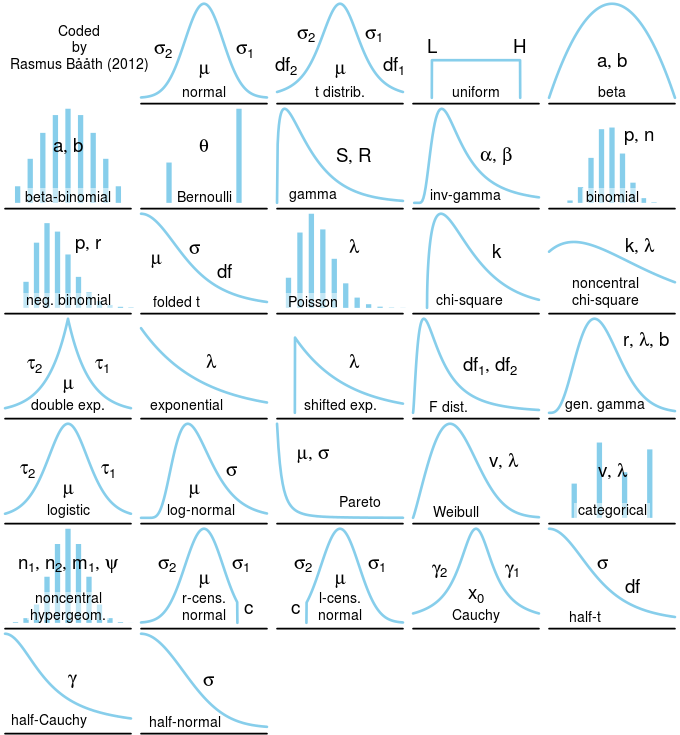
Figure 10.1: Probability distributions.
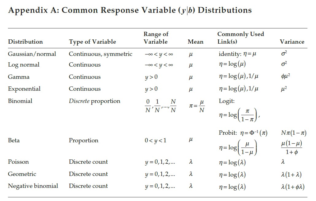
Figure 10.2: Properties of probability distributions.
10.4 Coming next
- Schedule your weekly/by-weekly meeting!
- Please fill out this form by Monday midnight.
- What’s coming next:
- Meet by appointment
- Potentially schedule group meetings for common topics