Day 7 Non-linear mixed models
February 5th, 2026
7.1 The general linear model
\[\mathbf{y} \sim N(\boldsymbol\mu, \boldsymbol\Sigma),\]
where:
- \(\mathbf{y} \equiv [y_1, y_2, \dots, y_n]'\) contains the response data,
- \(\boldsymbol{\mu} \equiv [\mu_1, \mu_2, \dots, \mu_n]'\) contains the expected values of said data,
- \(\boldsymbol\Sigma\) is the variance-covariance matrix.
The most typical model typically has:
- \(\boldsymbol\mu = \mathbf{X}\boldsymbol{\beta}\) and
- \(\boldsymbol\Sigma = \sigma^2\mathbf{I}\).
We can write the default model in most software written above as:
\[\mathbf{y} \sim N(\boldsymbol{\mu}, \Sigma),\\ \begin{bmatrix}y_1 \\ y_2 \\ y_3 \\ y_4 \\ \vdots \\ y_n \end{bmatrix} \sim N \left( \begin{bmatrix}\mu_1 \\ \mu_2 \\ \mu_3 \\ \mu_4 \\ \vdots \\ \mu_n \end{bmatrix}, \sigma^2 \begin{bmatrix} 1 & 0 & 0 & 0 & \dots & 0 \\ 0 & 1 & 0 & 0 & \dots & 0 \\ 0 & 0 & 1 & 0 & \dots & 0 \\ 0 & 0 & 0 & 1 & \dots & 0 \\ \vdots & \vdots & \vdots & \vdots & \ddots & \vdots\\ 0 & 0 & 0 & 0 & \dots & 1 \end{bmatrix} \right),\]
which is the same as
\[\begin{bmatrix}y_1 \\ y_2 \\ y_3 \\ y_4 \\ \vdots \\ y_n \end{bmatrix} \sim N \left( \begin{bmatrix}\mu_1 \\ \mu_2 \\ \mu_3 \\ \mu_4 \\ \vdots \\ \mu_n \end{bmatrix}, \begin{bmatrix} \sigma^2 & 0 & 0 & 0 & \dots & 0 \\ 0 & \sigma^2 & 0 & 0 & \dots & 0 \\ 0 & 0 & \sigma^2 & 0 & \dots & 0 \\ 0 & 0 & 0 & \sigma^2 & \dots & 0 \\ \vdots & \vdots & \vdots & \vdots & \ddots & \vdots\\ 0 & 0 & 0 & 0 & \dots & \sigma^2 \end{bmatrix} \right).\]
In summary, the assumptions are:
- Linearity
- Normality
- Independence
- Constant variance
7.2 Revisiting linearity
- Assume that \(y_i \sim N(\mu_i, \sigma^2)\).
…and there are 4 possible descriptions of the mean:
- \(\mu_i = \beta_0 + \beta_1 x_{1i} + \beta_2 x_{2i}\)
- \(\mu_i = \beta_0 + \beta_1 x_i + \beta_2 x_i^2\)
- \(\mu_i = \beta_0 \cdot \exp(x_i \cdot \beta_1)\)
- \(\mu_i = \beta_0 + x_i^{\beta_1}\)
What is a linear model and what is not?
7.3 Some benefits of non-linear models
- Process-based models versus non-process based models
- Process-based models are required to manage ecological systems in a changing world
Some agronomy examples:
7.4 Applied example
url <- "https://raw.githubusercontent.com/stat799/spring2026/refs/heads/main/data/N_fert.csv"
data_N <- read.csv(url) |>
  mutate(sy = factor(sy))

data_N |>
  ggplot(aes(Total_N, Yield_SY))+
  geom_point(aes(fill = sy),size=2.5, shape = 21)+
  scico::scale_fill_scico_d()+
  labs(x = expression(N[fert]~(kg~ha^{-1})),
       y = expression(Yield~(kg~ha^{-1})),
       fill = "Site-Year")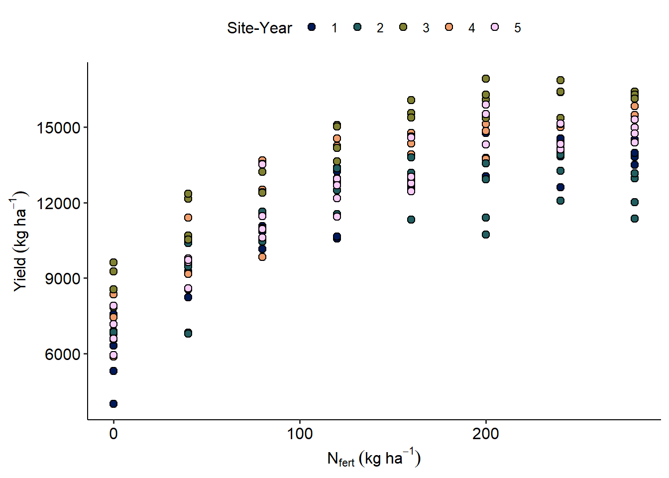
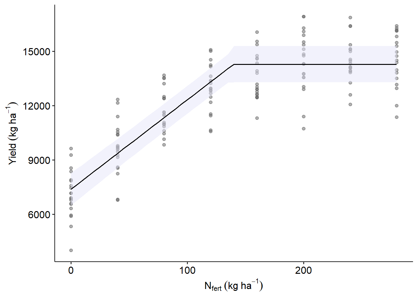
m1 <-
  nls(Yield_SY ~ Ymax - s * pmax(Ncrit - Total_N, 0),
    start = list(Ncrit = 150, Ymax = 14000, s =100),
    data = data_N)

m2 <-
  nls(Yield_SY ~ Ymax[sy] - s[sy] * pmax(Ncrit[sy] - Total_N, 0),
    start = list(Ncrit = rep(150, n_distinct(data_N$sy)),
                 Ymax = rep(14000, n_distinct(data_N$sy)),
                 s = rep(100, n_distinct(data_N$sy))),
    data = data_N)

library(nlme)
m3 <-
  nlme(Yield_SY ~ Ymax - s * pmax(Ncrit - Total_N, 0),
       data = data_N,
       fixed = Ncrit + Ymax + s ~ 1,
       random = Ncrit + Ymax + s ~ 1 | sy,
       start = c(Ncrit = 150, Ymax = 14000, s =100))
df_pred <- expand.grid(Total_N = seq(min(data_N$Total_N),
max(data_N$Total_N),by=5))
library(marginaleffects)## Warning: package 'marginaleffects' was built under R version 4.4.3## Please cite the software developers who make your work possible.
## One package: citation("package_name")
## All project packages: softbib::softbib()##
## Attaching package: 'marginaleffects'## The following object is masked from 'package:glmmTMB':
##
## refit## The following object is masked from 'package:lme4':
##
## refit## Warning: These arguments are not known to be supported for models of class `nlme`: level. All arguments are still passed to the
## model-specific prediction function, but users are encouraged to check if the argument is indeed supported by their modeling package.
## Please file a request on Github if you believe that an unknown argument should be added to the `marginaleffects` white list of known
## arguments, in order to avoid raising this warning: https://github.com/vincentarelbundock/marginaleffects/issuesas.data.frame(y_pred) |>
ggplot(aes(Total_N, estimate))+
geom_point(aes(Total_N, Yield_SY),alpha =.5,
data = data_N, color = "grey40")+
geom_ribbon(aes(ymin = conf.low, ymax = conf.high),alpha =.5,
fill = "lavender")+
geom_line()+
labs(x = expression(N[fert]~(kg~ha^{-1})),
y = expression(Yield~(kg~ha^{-1})))