Day 8 Statistical inference
February 6th, 2026
8.1 What is statistical inference?
- “Use math to understand the world”
- From raw data to assumptions to understanding (?)
- Define target population
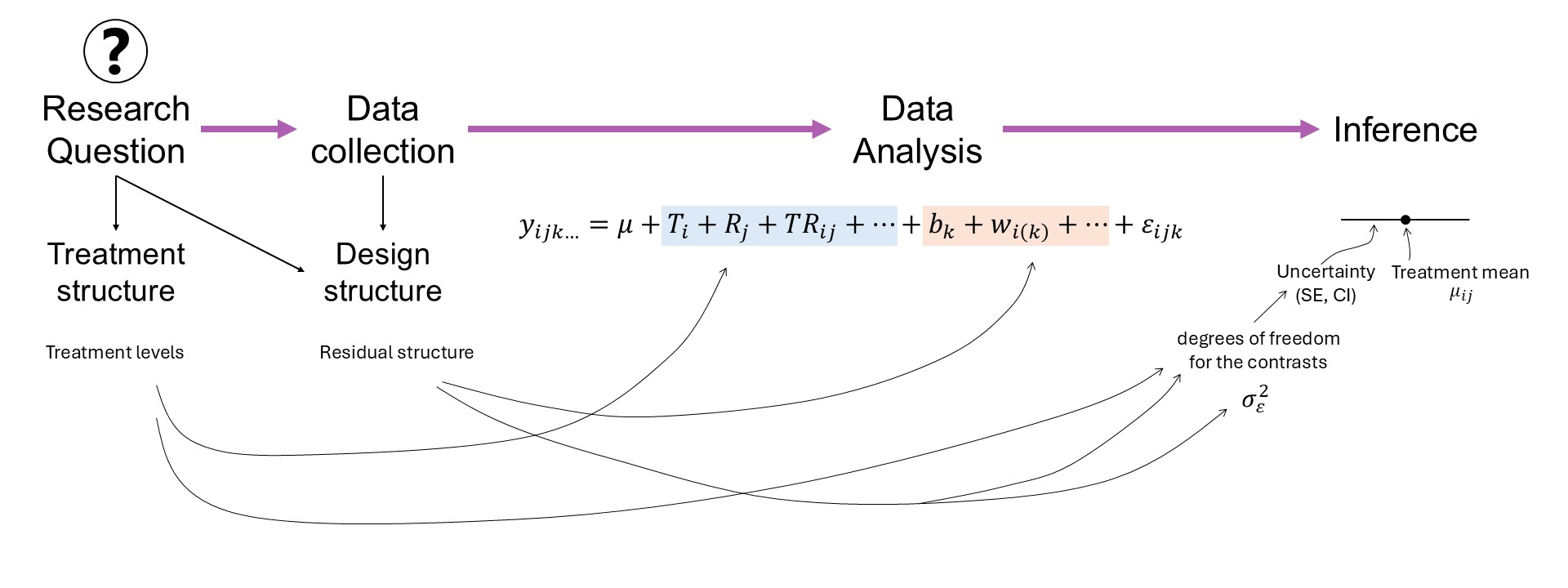
Figure 8.1: Mind map in a research project.
8.2 The components that go into interpreting results (in the context of LMMs)
8.2.1 Estimation
- Uncertainty in estimation – where is it coming from?
- Contrasts
- Multiple comparisons
Let’s revisit the Nitrogen example, where we describe yield \(y_{ij}\) (\(i\)th observation in \(j\)th location) as
\[y_{ij} \sim N(\mu_{ij}, \sigma^2), \\ \mu_{ij} = \beta_{0j} + \beta_1 x_{ij} + \beta_2 x_{ij}^2. \]
url <- "https://raw.githubusercontent.com/stat799/spring2026/refs/heads/main/data/N_fert.csv"
data_N <- read.csv(url) |> mutate(sy = as.factor(sy))

data_N |>
  ggplot(aes(Total_N, Yield_SY))+
  geom_point(size=2.5)+
  labs(x = expression(N[fert]~(kg~ha^{-1})),
       y = expression(Yield~(kg~ha^{-1})))+
  theme_pubr()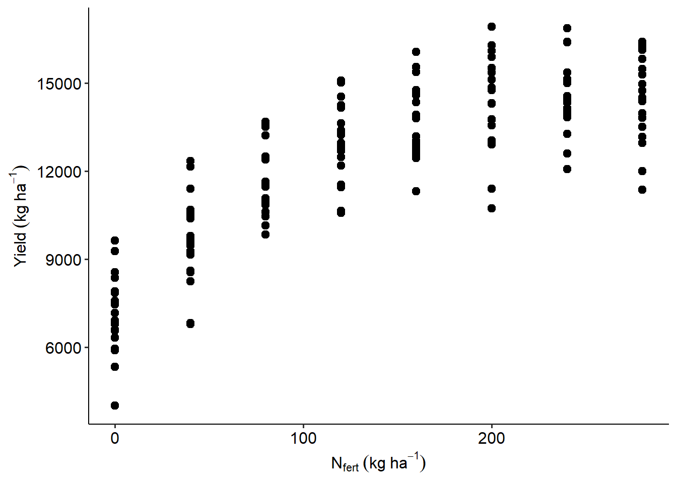
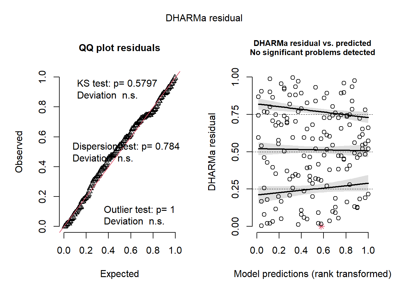
## Object of Class DHARMa with simulated residuals based on 250 simulations with refit = FALSE . See ?DHARMa::simulateResiduals for help.
##
## Scaled residual values: 0.168 0.54 0.004 0.904 0.764 0.428 0.02 0.18 0.596 0.868 0.744 0.744 0.352 0.748 0.116 0.676 0.08 0.256 0.46 0.768 ...
There’s multiple aspects to consider when we want to interpret the data.
What was the main objective of the study?
Option A: Study the effect of N on yield
- Consider the mean \(f(x) = \mu_{ij} = \beta_{0j} + \beta_1 x_{ij} + \beta_2 x_{ij}^2\).
- The slope is then \(f'(x) = \beta_1 + 2 \beta_2 x_{ij}\)
- The slope depends on the level of \(N_{fert}\) we are considering!
- Likewise, consider \(se(\hat{\beta}_1 + 2 \hat{\beta}_2 x_{ij})\).
- How can we estimate the variance of a combination of parameters?
- The delta method sets the asymptotic variance of a function \(g(\cdot)\) of the parameters (\(g(\hat\beta)\)): \(Var(g(\hat\beta)) \approx \nabla g(\hat\beta)^T Cov(\hat\beta) \nabla g(\hat\beta),\) where \(\nabla g(\hat\beta)\) is the gradient (vector of first derivatives) of function \(g(\cdot)\) with respect to the parameters.
- In this case \(se(\hat{\beta}_1 + 2 \hat{\beta}_2 x_{ij}) = \sqrt(\widehat{Var}(\hat\beta_1)+ 4 x_{ij}^2\widehat{Var}(\hat\beta_2) + 4x_{ij}\widehat{Cov}(\hat\beta_2))\)
##                (Intercept)       Total_N  I(Total_N^2)           sy2           sy3           sy4           sy5
## (Intercept)   53465.012101 -4.143965e+02  1.148989e+00 -2.762121e+04 -2.762121e+04 -2.787241e+04 -2.762121e+04
## Total_N        -414.396458  8.777726e+00 -2.908876e-02  5.914528e-14  5.353022e-14 -7.348210e+00  3.743372e-14
## I(Total_N^2)      1.148989 -2.908876e-02  1.044085e-04 -2.632058e-16 -2.310362e-16  4.571248e-02 -1.754706e-16
## sy2          -27621.209876  5.914528e-14 -2.632058e-16  5.524242e+04  2.762121e+04  2.762121e+04  2.762121e+04
## sy3          -27621.209876  5.353022e-14 -2.310362e-16  2.762121e+04  5.524242e+04  2.762121e+04  2.762121e+04
## sy4          -27872.409930 -7.348210e+00  4.571248e-02  2.762121e+04  2.762121e+04  5.714695e+04  2.762121e+04
## sy5 -27621.209876 3.743372e-14 -1.754706e-16 2.762121e+04 2.762121e+04 2.762121e+04 5.524242e+04## [1] 2.962723## [1] 1.148286## [1] 1.487304We can also do this with the emmeans package:
##  Total_N Total_N.trend   SE  df lower.CL upper.CL
##        0         61.99 2.96 151    56.14     67.8
##      100         35.88 1.15 151    33.62     38.1
##      200          9.77 1.49 151     6.83     12.7
##
## Results are averaged over the levels of: sy
## Confidence level used: 0.95
Option B: Study the effect of N on yield
- If we set \(f'(x) =0\) and solve for \(x\), we can get the optimum rate.
- \(ONR = -\frac{\beta_1}{2\beta_2}\)
- Consider the uncertainty behind \(-\frac{\beta_1}{2\beta_2}\).
##  Total_N
## 237.5568
Same thing, we can get SE using the delta method:
## [1] 8.3076688.2.2 Prediction
- Uncertainty in predictions
- Conditional distribution
- Marginal distribution
Recall
\[y_{ij} \sim N(\mu_{ij}, \sigma^2), \\ \mu_{ij} = \beta_{0j} + \beta_1 x_{ij} + \beta_2 x_{ij}^2. \]
Where is the uncertainty coming from?
How can the uncertainty change depending on how \(\beta_{0j}\) is specified?
Model evaluation criteria for prediction-oriented models
8.3 On the use of R2 for statistical inference
Why do so many people use the coefficient of variation R2?
- Metrics like RMSE are hard to compare across models (different units)
- R2, however, is dimensionless and much easier to interpret
- “The proportion of variability that is explained by the model”
R2 can be computed as
\[R^2 = \frac{SSM}{SST} = \frac{SS_{MODEL}}{SS_{INT-SLOPE}} = 1 - \frac{SSE}{SST},\]
where \(R^2\) is the coefficient of variation, \(SSM\) is the sum of squares of the model, \(SST\) is the total sum of squares (i.e., the residual sum of squares of an intercept-and-slope model). In essence, \(R^2\) is the ratio between the \(SSE\) of whatever model and the \(SSE\) of an intercept-and-slope model.
Uncertainty in R2
## [1] 0.89665928.3.1 Bootstrapped R2
boot_r2 <- do(1000) * {
  m_boot <- lm(Yield_SY ~ Total_N + I(Total_N^2),
               data = resample(data_N, size = nrow(data_N), replace = TRUE))

  summary(m_boot)$r.squared
}

hist(boot_r2$result)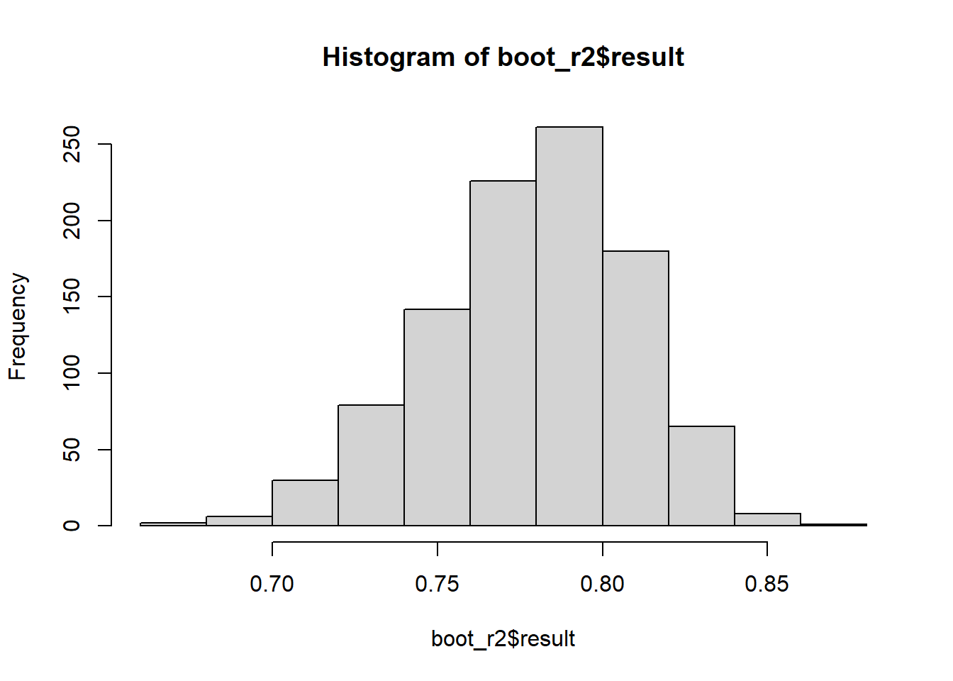
8.3.2 Out-of-sample R2
R2_oos <- numeric()

for (i in unique(data_N$sy)) {
  # leave-one-sy-out
  d_is <- data_N |> filter(sy != i)
  d_oos <- data_N |> filter(sy == i)

  m <- lm(Yield_SY ~ Total_N + I(Total_N^2), data = d_is)

  SST_oos <- sum((resid(lm(Yield_SY ~ 1, data =d_oos)))^2)
  SSE_oos <- sum((d_oos$Yield_SY - predict(m, newdata = d_oos))^2)

  R2_oos[i] <- 1 - SSE_oos/SST_oos

}

R2_oos
## 1 4 2 3 5
## 0.7341245 0.8376546 0.3494678 0.3219911 0.9103108## [1] 0.6307098## [1] 0.2766323- Compare the R2